Eshelby's tensor

Introduction

The purpose of this post is to expound upon the fundamental tensors that arise within the Eshelby’s problem, offering their concise closed forms. While the tedious derivations are omitted here, I supplement this with finite element simulations to validate the equations. Included are Matlab/Octave codes designed to compute the Eshelby’s tensors for arbitrary ellipsoids and anisotropic materials. These codes may prove particularly valuable in coding self-consistent polycrystal homogenization approaches.

Eshelby’s problem centers around an ellipsoidal inclusion embedded within an infinitely large homogeneous matrix. When the inclusion alters its dimensions or form through the imposition of eigen strains (such as thermal or phase-induced strains), it prompts stress formation both within the inclusion and its surroundings. Remarkably, Eshelby demonstrated that stress (and strain) within the ellipsoidal inclusion remains uniform.

The correlation between the applied eigen strain $\varepsilon_{ij}^0$ within the ellipsoidal domain and the ensuing strain $\varepsilon_{ij}$ generated within this domain is described by the equation:

\[\varepsilon_{ij} = S_{ijkl}\varepsilon_{kl}^0\]

where $S_{ijkl}$ is the fourth order Eshelby’s tensor. Beginning with the most general case of the Eshelby’s tensor in the following section, I then proceed with simpler cases developed under certain specific assumptions.

Fully anisotropic material

Let’s begin with the implicit equation of an ellipsoid:

\[\left(\frac{x_1}{a_1}\right)^2 + \left(\frac{x_2}{a_2}\right)^2 + \left(\frac{x_3}{a_3}\right)^2 = 1\]

where $x_i$ are the coordinates along the principal axes and $a_i$ are the lengths of the semi-axes.

In the case of a fully anisotropic material, the Eshelby’s tensor cannot be derived in a closed form but can be expressed in terms of elliptical integrals that can be solved numerically. This most general form is expanded in the text below.

Let us first define the Hill polarization tensor $P_{ijkl}$ in the form presented by (Masson 2008), (Suvorov and Dvorak 2002).

\[P_{ijkl} = \frac{1}{4\pi} \int_{\theta=0}^{\pi}\int_{\phi=0}^{2\pi} M_{ijkl}(\theta,\phi)\sin\theta d\theta d\phi \label{eq:hill_polarization_tensor}\]

where

\[M_{ijkl} = \frac{1}{4}\left(A_{jk}^{-1}\xi_i\xi_l + A_{ik}^{-1}\xi_j\xi_l + A_{jl}^{-1}\xi_i\xi_k + A_{il}^{-1}\xi_j\xi_k\right)\]

Note that in the previous equation, $A_{jk}^{-1}$ indicate the elements of the inverse matrix.

Let us then define a vector $\vec{\xi}$ given by:

\[\begin{split} \xi_1 &= \frac{\sin\theta \cos\phi}{a_1}\\ \xi_2 &= \frac{\sin\theta \sin\phi}{a_2}\\ \xi_3 &= \frac{\cos\phi}{a_3}\\ \end{split}\]

and a tensor:

\[A_{ik} = C_{ijkl}\xi_j\xi_l\]

The Eshelby’s tensor can then be obtained by the multiplication of the Hill polarization tensor $P_{ijkl}$ and the tensor of elastic constants $C_{ijkl}$:

\[S_{ijkl} = P_{ijmn}C_{mnkl}\]

Having established the Eshelby’s tensor, it is now possible to calculate the strain $\boldsymbol{\varepsilon}$ within the ellipsoid given its eigen strain $\boldsymbol{\varepsilon}^0$. Notice however, that for a fully anisotropic case, numerical integration needs to be employed to evaluate the previous equations. One possible implementation is discussed below.

Numerical Integration - Gauss-Legendre Quadrature

The integration of the previous equations can be approximated by the Gauss integration scheme:

\[\frac{1}{4\pi}\int_{\theta=0}^{\pi}\int_{\phi=0}^{2\pi} M_{ijkl}(\theta,\phi)\sin\theta d\theta d\phi \approx \frac{1}{4\pi} \sum_i\sum_j M_{ijkl}(\theta_i,\phi_i)\sin \left(\theta_i\right) w_iw_j \det \boldsymbol{J}\]

where $\theta = \frac{\pi}{2}(\xi+1)$ and $\phi = \pi(\eta+1)$ and the Jacobian of the transformation is

\[\boldsymbol{J} = \begin{bmatrix} \frac{\partial \theta}{\partial \xi} & \frac{\partial \theta}{\partial \eta} \\ \frac{\partial \phi}{\partial \xi} & \frac{\partial \phi}{\partial \eta} \end{bmatrix} = \begin{bmatrix} \frac{\pi}{2} & 0 \\ 0 & \pi \end{bmatrix}\]

therefore $\det \boldsymbol{J} = \frac{\pi^2}{2}$.

In the previous expressions, $w_i$ are the Gauss weights and $\xi$ and $\eta$ are the Gauss node coordinates.

A Matlab code evaluating the Eshelby’s tensor for arbitrary aspect ratio and anisotropy is given below:

Finite element simulation - verification of the semi-analytical implementation

Due to the intricate and error-prone nature of deriving the aforementioned equations, ensuring our confidence in their application necessitates a finite element simulation. This approach involves comparing the outcomes of a numerical finite element simulation solution with the semi-analytical solution outlined by the previous equations.

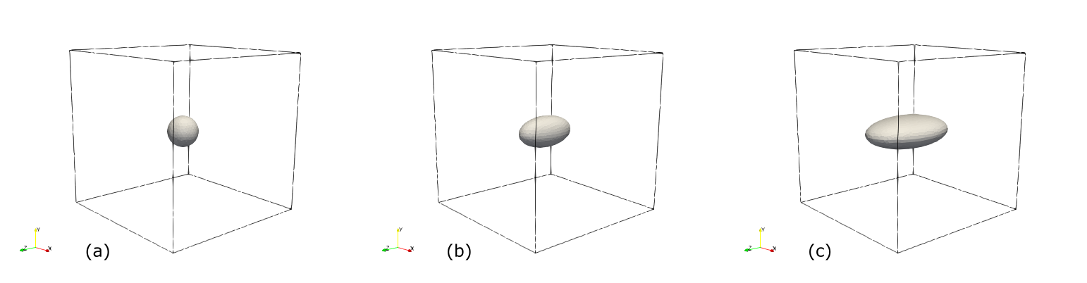
A finite element analysis is constructed encompassing three distinct cases of ellipsoids characterized by aspect ratios $a\times b\times c$: $1\times 1\times 1$, $1\times 1 \times 2$, and $2 \times 1\times 3$.

The finite element Representative Volume Elements (RVEs) are visually depicted below. It’s worth noting that these RVEs possess finite dimensions, which stands in contrast to the Eshelby solutions derived for an infinitely large matrix. Consequently, this discrepancy may introduce some variations. However, as long as the matrix’s dimensions are sufficiently large relative to the size of the ellipsoid, any resulting error should remain relatively minor.

Let us generate a random eigen strain tensor

\[\boldsymbol{\varepsilon}_0 = \begin{bmatrix} 0.023522 & 0.076558 & 0.019838 & 0.068208 & 0.059107 & 0.031905 \end{bmatrix}^T\]

Given this eigen strain, the strain generated within the ellipsoid is predicted using the semi-analytical solution (see Matlab code) and using the finite element simulation. The results are compared in the table below.

	$\boldsymbol{\varepsilon}_0$	1x1x1		1x1x2		2x1x3
		FEM	analytical	FEM	analytical	FEM	analytical
$xx$	0.023522	0.016544	0.016907	0.0197261	0.020092	0.0106386	0.009391
$yy$	0.076558	0.042158	0.042171	0.0507705	0.050056	0.0676905	0.067769
$zz$	0.019838	0.014737	0.015157	0.0064683	0.006845	0.0050078	0.0051844
$yz$	0.068208	0.032787	0.032480	0.0316119	0.030895	0.0429553	0.04018
$zx$	0.059107	0.028448	0.028146	0.0273814	0.026772	0.0220308	0.019031
$xy$	0.031905	0.015371	0.015187	0.0184856	0.018011	0.0208782	0.018065

An important observation to make is that in the isotropic scenario, the outcomes remain unaffected by the Young’s modulus $E$, manifesting a dependency solely on the Poisson’s ratio $\nu$.

To illustrate the convergence of the semi-analytical solutions across varying numbers of Gauss integration points towards the numerical finite element solution, refer to the figures provided below. These figures distinctly demonstrate the alignment between the results. The dashed lines in the figures represent the finite element simulation solutions for the six components of the strain tensor, while the circled lines represent the semi-analytical solutions for varying number of Gauss integration points with increased number of integration points leading to a more precise result.

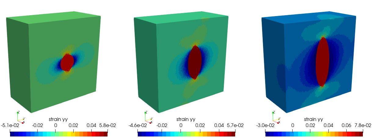
Below, the outcomes of the finite element simulations for the three outlined cases are displayed. These visualizations depict the $\varepsilon_{yy}$ component of the strain field, effectively illustrating the uniform nature of strain (and stress) within the ellipsoid. This corroborates the findings derived by Eshelby. A notable observation is the remarkable concurrence between the numerical outcomes and the semi-analytical solutions derived for an infinitely extensive matrix, despite the presence of stress-free boundaries.

In the ultimate assessment, the case involving dimensions $2 \times 1 \times 3$ is explored, featuring a random eigen strain $\varepsilon_{ij}^0$ coupled with a fully anisotropic tensor of elastic constants $C_{ijkl}$. Importantly, when generating a random elastic tensor matrix, it’s imperative to verify its positive definiteness. For instance using Matlab, this can be accomplished by employing the ‘chol(C)’ function, which would issue an error message if matrix ‘C’ lacks positive definiteness.

For the following case of eigen strain and tensor of elastic constants

\[\boldsymbol{\varepsilon}_0 = \begin{bmatrix} 0.023522 & 0.076558 & 0.019838 & 0.068208 & 0.059107 & 0.031905 \end{bmatrix}^T\] \[\boldsymbol{C} = \begin{bmatrix} 1.9627 & 0.71094 & 1.2973 & 2.1394 & 1.908 & 1.1079 \\ & 0.88304 & 0.57145 & 1.129 & 0.85012 & 0.76032 \\ & & 1.7383 & 1.7461 & 1.5757 & 0.97334 \\ & & & 2.8236 & 2.6732 & 1.5282 \\ & & & & 2.9695 & 1.4951 \\ & & & & & 1.1461 \\ \end{bmatrix}\]

the results of the semi-analytical and numerical solutions are collated in the figure below. Also, strain field within and around the ellipsoidal inclusion is presented.

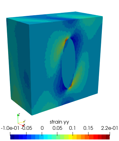
A noteworthy observation is the heightened complexity of the strain field surrounding the precipitate and reaching the domain boundaries. In terms of the semi-analytical solution, it becomes evident that an increased number of Gauss integration points would facilitate even stronger convergence. Nevertheless, it is evident that the semi-analytical results and the finite element simulation outcomes align remarkably well also for a case of a fully anisotropic material.

Special cases - closed form solutions

The previous section explored an arbitrary ellipsoid within an anisotropic material. However, by imposing specific assumptions about the ellipsoid’s shape and considering simplified anisotropic conditions, it is possible to derive closed-form analytical solutions. Several of such examples are considered below:

Isotropic sphere

For the case of a spherical inclusion and isotropic material, the following expression can be derived (Hutchinson and Hill 1970):

\[S_{ijkl} = \left(1-\frac{5}{3}\beta\right)I_{ij}I_{kl} + \frac{1}{2}\beta \left(I_{ik}I_{jl} + I_{il}I_{jk} - \frac{2}{3}I_{ij}I_{kl}\right)\]

where $\beta = \frac{10\nu -8}{15(\nu-1)}$

Below is a Matlab code. You can easily verify that the outcomes of both the general code and this specific code will align when dealing with an isotropic spherical inclusion.

2D elliptical isotropic inclusion

For a 2D case of an elliptical inclusion (or a cylinder in 3D) and isotropic material, the following can be derived. As highlighted earlier, in the isotropic case, the Eshelby’s tensor depends only on the Poisson’s ratio $\nu$:

\[\begin{split} S_{1111} &= \frac{a_2\left[2(1-\nu)(a_1+a_2)+a_1\right]}{2(1-\nu)(a_1+a_2)^2}\\ S_{2222} &= \frac{a_1\left[2(1-\nu)(a_1+a_2)+a_2\right]}{2(1-\nu)(a_1+a_2)^2}\\ S_{3333} &= 0\\ S_{1122} &= \frac{a_2\left[-(1-2\nu)a_1+2\nu a_2\right]}{2(1-\nu)(a_1+a_2)^2}\\ S_{2211} &= \frac{a_1\left[-(1-2\nu)a_2+2\nu a_1\right]}{2(1-\nu)(a_1+a_2)^2}\\ S_{1133} &= \frac{\nu a_2}{(1-\nu)(a_1+a_2)}\\ S_{3311} &= 0\\ S_{1313} &= \frac{a_2(2-\nu)}{2(1-\nu)(a_1+a_2)}\\ S_{2323} &= \frac{a_1(2-\nu)}{2(1-\nu)(a_1+a_2)}\\ \end{split}\]

Finally, symmetries are applied: \(S_{ijkl} = S_{ijkl} = S_{ijlk} = S_{jilk}\)

A Matlab code is provided below:

References

::: {#refs .references .hanging-indent} ::: {#ref-doi:10.1098/rspa.1970.0177} Hutchinson, J. W., and Robert Hill. 1970. “Elastic-Plastic Behaviour of Polycrystalline Metals and Composites.” Proceedings of the Royal Society of London. A. Mathematical and Physical Sciences 319 (1537): 247–72. https://doi.org/10.1098/rspa.1970.0177. :::

::: {#ref-MASSON2008757} Masson, Renaud. 2008. “New Explicit Expressions of the Hill Polarization Tensor for General Anisotropic Elastic Solids.” International Journal of Solids and Structures 45 (3): 757–69. https://doi.org/https://doi.org/10.1016/j.ijsolstr.2007.08.035. :::

::: {#ref-SUVOROV20025659} Suvorov, Alexander P., and George J. Dvorak. 2002. “Rate Form of the Eshelby and Hill Tensors.” International Journal of Solids and Structures 39 (21): 5659–78. https://doi.org/https://doi.org/10.1016/S0020-7683(02)00369-4. ::: :::